Stochastic – Differential Chapman-Kolmogorov Equation

Posted on March 28, 2017April 20, 2017 by teracamo

Introduction

Here we do not show the derivation of Differential Chapman-Kolmogorov Equation, instead, we only show how to interpret the result. In the following sections, it is assumed that the stochastic process has Markov properties and the sample paths are always continuous and satisfy [Eq.1]:

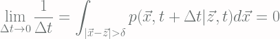
$\displaystyle \lim_{\Delta t \rightarrow 0} \frac{1}{\Delta t} = \int_{|\vec{x}-\vec{z}| > \delta} p(\vec{x}, t+\Delta t|\vec{z}, t) d\vec{x} = 0$

which practically says that integrating all possibility of changes of states z to x (i.e. the “distance”) that are greater than δ with δ > 0, the result probability is zero and, thus, there are no possibility that there are any changes of states within an infinitesimal period of time Δt. This is also called the Lindeberg condition.

Chapman-Kolomogov Equation

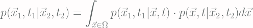
The Chapman-Kolomogov Equation defines, for a Markov Process, the conditional probabilities [Eq.2]:

$\displaystyle p(\vec{x}_1, t_1|\vec{x}_2, t_2) = \int_{\vec{x} \in \Omega} p(\vec{x}_1, t_1|\vec{x}, t) \cdot p(\vec{x}, t| \vec{x}_2, t_2) d\vec{x}$

Differential Chapman-Kolomogov Equation

Assumptions

W.r.t that, we requires the following properties in order to reduce [Eq.2] into a differential equation for all δ > 0 and denote condition |x-z| < δ as ε:

$\displaystyle W(\vec{x}|\vec{z}, t)=\lim_{\Delta t \rightarrow 0} \frac{1}{\Delta t} \cdot p(\vec{x}, t+\Delta t|\vec{z}, t) \text{, for }|x-z| \geq \delta$

$\displaystyle A_i(\vec{z}, t) + O(\delta) = \lim_{\Delta t \rightarrow 0}\frac{1}{\Delta t} \int_{\epsilon} p(\vec{x}, t+\Delta t|\vec{z}, t) (x_i - z_i) d\vec{x}$

$\displaystyle B_{ij}(\vec{z}, t) + O(\delta) \\ \indent =\lim_{\Delta t \rightarrow 0} \frac{1}{\Delta t} \int_{\epsilon} p(\vec{x}, t+\Delta t|\vec{z}, t) (x_i - z_i)(x_j - z_j) d\vec{x}$

In the first requirement, W(z, t) is the jump term which describe discontinuous evolution for all +ve non-zero distance between x and z. Note that if W = 0, we restore [Eq.1] and the sample path is continuous.

In the second requirement, if δ limit to zero, the O(δ) term vanishes (i.e. continuous path), and the term A_i is often called the drift term because it suggest that E[dx] = A(x, t)dt, which can be interpret as the instantaneous rate of change of z..

In the third requirement, B(z, t) is often referred as the diffusion term, which can be seen as the instantaneous rate of change of covariance of all process close to z.

Derivation

The full derivation will not be stated here, in fact it can be easily found on the internet by search the key words Differential Chapman-Kolmogorov. However, it is crucial to understand the origin of it and a brief introduction to the origin of differential Chapman-Kolmogorov equation will be written below referencing Crispin Gardiner’s book Stochastic methods: a handbook for the natural and social sciences.

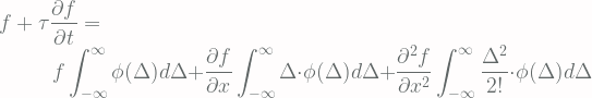
First, we consider the time evolution of certain function f(z) which we required it to be twice differentiable. Then the instantaneous rate of change of expected value of this function can be written as:

$\displaystyle \frac{\partial}{\partial t} \int_{\vec{x} \in \Omega} f(\vec{x})p(\vec{x}, t|\vec{y}, t') d\vec{x}$

$\displaystyle = \lim_{\Delta t \rightarrow 0} \left[ \frac{1}{\Delta t} \int_{\vec{x} \in \Omega} d\vec{x} \left\{ f(\vec{x}) \Big[p(\vec{x}, t+\Delta t|\vec{y}, t') - p(\vec{x}, t|\vec{y}, t') \Big] \right\} \right]$
[by first principle]

$\displaystyle = \lim_{\Delta t \rightarrow 0} \left[ \frac{1}{\Delta t} \int d\vec{x} \int d\vec{z} \left\{ f(\vec{x}) \Big[ p(\vec{x}, t+\Delta t|\vec{z}, t)p(\vec{z}, t|\vec{y}, t') - f(\vec{z})p(\vec{z}, t|\vec{y}, t') \Big] \right\} \right]$
[by Chapman-Kolmogorov Equation]

Divide the integrals into two regions |x-z| > δ and |x-z| < δ and some manipulation, the result will be [Eq.3]:

$\displaystyle \frac{\partial p(\vec{z}, t|\vec{y}, t')}{\partial t} = - \sum_i \frac{\partial}{\partial z_i} \big[ A_i(\vec{z}, t)p(\vec{z}, t|\vec{y}, t') \big] + \frac{1}{2} \sum_{i, j} \frac{\partial^2}{\partial z_i \partial z_j}\Big[B_{ij}(\vec{z}, t)p(\vec{z}, t|\vec{y}, t')\Big] \\ \indent + \int_{\vec{x} \in \Omega} \Big[ W(\vec{z}|\vec{x}, t)p(\vec{x}, t|\vec{y}, t') - W(\vec{x}|\vec{z}, t)p(\vec{z}, t|\vec{y}, t') \Big] d\vec{x}$

this is the differential Chapman-Kolmogorov equation or sometimes called the master equation

Interpreting the equation

Discontinuous jumps

If we deliberately force the master equation to disobey [Eq.1], we will obtain a discontinuous process. For example, forcing both A(z, t) and B(z, t) to be zero, the differential equation is left to be:

$\displaystyle \frac{\partial}{\partial t} p(\vec{z}, t|\vec{y}, t') = \int_{\vec{x} \in \Omega} d\vec{x} \Big[ W(\vec{z}|\vec{x}, t) p(\vec{x}, t|\vec{y}, t') - W(\vec{x}|\vec{z}, t)p(\vec{z}, t|\vec{y}, t')\Big]$

Using initial condition $p(\vec{z}, t|\vec{y}, t') = \delta(\vec{y} - \vec{z})$ , with delta being the Dirac-Delta function, the particular solution to the master equation is:

$\displaystyle p(\vec{z}, t+\Delta t|\vec{y}, t)$

$\displaystyle = \delta(\vec{y} - \vec{z})\Big[ 1 - \int_{\vec{x} \in \Omega} W(\vec{x}|\vec{y}, t)\Delta t d\vec{x}\Big] + W(\vec{z}|\vec{y}, t)\Delta t$

see that if we want to know the probability of staying in y after Δt, we substitute z as y and get the following equation [Eq.4]

$\displaystyle p(\vec{y}, t+\Delta t)|\vec{y}, t) = 1\Big[ 1-\int_{\vec{x} \in \Omega} W(\vec{x}|\vec{y}, t)\Delta t d\vec{x} \Big] + W(\vec{y}|\vec{y}, t)\Delta t$

Let’s break this down terms by terms so that it is easier to understand. Firstly, W(z|y, t) is the instantaneous probability (or probability per time) of going to state z from y, therefore, W(z|y, t)Δt is the accumulated probability of going to z from y within time period Δt. Secondly, the integral inside the square bracket denotes the total probability of leaving state y and going to any other states x, thus, one minus the integral is the total probability of staying in state y. In the case of [Eq.4], W(y|y, t)Δt is the probability of going from state y to state y meaning it includes the probability of first leaving state y then go back to y within Δt, and the integral represents ONLY staying in state y. Finally, the sum of both terms converge to the probability of staying in state y within Δt in [Eq.4].

Fokker-Planck Equation

The Fokker-Planck Equation is obtained when forcing the Jump term W in the master equation to become zero [Eq.5]

This equation is sometimes know as the diffusion process with drift term A and diffusion matrix B. Based on this equation, if we wish to compute $p(\vec{z}, t+\Delta t|\vec{y}, t')$ , we can neglect the partial derivatives of A and B so that equation [Eq.5] becomes:

$\displaystyle \frac{\partial p(\vec{z}, t|\vec{y}, t')}{\partial t} = - \sum_i A_i(\vec{z}, t)\frac{\partial}{\partial z_i} \big[ p(\vec{z}, t|\vec{y}, t') \big] + \frac{1}{2} \sum_{i, j} B_{ij}(\vec{z}, t) \frac{\partial^2}{\partial z_i \partial z_j}\Big[p(\vec{z}, t|\vec{y}, t')\Big]$

and solve this equation with the constrain $p(\vec{z}, t|\vec{y}, t) = \delta(\vec{z} - \vec{y})$ (i.e. only one state exist at a time) and obtain:

$\displaystyle p(\vec{z}, t+\Delta t|\vec{y}, t) = \sqrt{\Big[(2\pi)^N \text{det}(B(\vec{y}, t)\Delta t) \Big]}^{-1} \cdot \\ \indent \exp \bigg[ -\frac{1}{2\Delta t} [\vec{z}-\vec{y}-A(\vec{y}, t)\Delta t]^T B(\vec{y}, t)^{-1} [\vec{z} - \vec{y} - A(\vec{y}, t)\Delta t]\bigg]$

which is, in fact, a Gaussian distribution with variance as matrix $B$ and mean $\vec{y} + A(\vec{y}, t)\Delta t$ .

Reference

Crispin W.. Gardiner. Stochastic methods: a handbook for the natural and social sciences. Springer, 2009.

Hierro, Juan, and César Dopazo. “Singular boundaries in the forward Chapman-Kolmogorov differential equation.” Journal of Statistical Physics 137.2 (2009): 305-329.

Stochastic Differential Equation with Applications

Learning Notes

Stochastic – Shot Noise

Posted on March 24, 2017March 27, 2017 by teracamo

Definition of Problem

To model probability distribution P(X=n, t) of noises caused by random arrival of electrons in a vacum tube.

Annotation

λ = Probability constant of electron arrive over a period of time, intensity of Poisson Dist.

n = Total number of electrons arrived at time t

G = Generating function

Derivation

Let P(n, t) be the probability of a total of n electrons arrived at time t. The probability of an electron arriving over a period Δt can be modulated by a constant λ:

$\displaystyle P(n+1, t+\Delta t) - P(n, t) = \lambda \Delta t$

Then the probability of having n arrival at t + Δt is the sum of probabilities: 1) Already has n arrival and no arrivals in Δt. 2) Already has n – 1 arrival and one arrivals in Δt. Formulated as follow:

$\displaystyle P(n, t+ \Delta t) = P(n, t)(1 - \lambda \Delta t) + P(n-1, t)(\lambda \Delta t)$

Re-arrange the upper equation we get [Eq.1]

$\displaystyle \frac{\partial P(n, t)}{\partial t} = \frac{P(n, t+\Delta t) - P(n, t)}{\Delta t} = \lambda \left[P(n- 1, t) - P(n, t)\right]$

At this point, we would like to introduce a math skill Generating Function and denotes:

$\displaystyle G(s, t) = \sum_n^{\infty} s^n P(n, t)$

so that:

$\displaystyle \frac{\partial G(s, t)}{\partial t} = \sum_n^{\infty} s^n \frac{\partial P(n, t)}{\partial t}$

$\displaystyle = \lambda \sum_{n=0}^{\infty} s^n \left[P(n-1, t) - P(n, t)\right]$

$\displaystyle = s \cdot \sum_{n=-1}^{\infty} s^n P(n, t)-\sum_{n=0}^{\infty} P(n, t)$

$\displaystyle = s \cdot \sum_{n=0}^{\infty} s^n P(n, t)-\sum_{n=0}^{\infty} P(n, t)$
[P(-1, t) = 0 for all t since number of arrival must not be negative]

$\displaystyle = \lambda(s - 1) \sum_{n=0}^{\infty} s^n P(n, t)$

$= \lambda(s-1) \cdot G(s, t)$

We then get ourselves a p.d.e:

$\displaystyle \frac{\partial G}{\partial t} = \lambda (s-1) G$

separating variables,

$\displaystyle \frac{\partial G}{G} = \lambda (s-1) \partial t$

$\displaystyle \ln{[G(s, t)]} = \lambda t(s-1) + C$

With the initial condition of G(s, 0) being 1 because P(0, 0) = 1 and P(n, 0) = 0 for all n, the particular solution would be:

$\displaystyle G(s, t) = e^{\lambda t(s-1)}G(s, 0)$

Perform Taylor expansion at s = 0:

$\displaystyle G(s, t) = G(0, t) + s\cdot\frac{G'(0, t)}{1!} + s^2 \cdot \frac{G''(0, t)}{2!} + \cdots$

$\displaystyle \sum_n^{\infty} s^n P(n, t) = e^{-\lambda t} + \frac{s}{1!}\cdot(\lambda t)e^{-\lambda t} + \frac{s^2}{2!} e^{-\lambda t}$

By comparing terms in powers of s, we can deduce:

$\displaystyle P(n, t) = \frac{(\lambda t )^n e^{-\lambda t}}{n!}$

which is actually a Poisson Process.

Useful equations

Posted on March 23, 2017April 24, 2017 by teracamo

Taylor Series

$\displaystyle f(x) = f(a) + \frac{f'(a)}{1!}(x - a) + \frac{f''(a)}{2!} (x-a)^2 + \cdots$

$\displaystyle f(x) = \sum_{n=0}^{\infty} \frac{f^{(n)}(a)}{n!}(x-a)^n$

Bra-kets Notation

$\displaystyle \langle m | n \rangle = \delta_{m,n}$

$\displaystyle \sum_n | n \rangle \langle n| = I$

Probabilities

Bayes’ theorem

$\displaystyle P(A|B) = \frac{P(B|A)P(A)}{P(B)}$

Mean/Expectation value

For x being an event mapped by random variable X
$\displaystyle \left<X\right> = \sum_{x \in \Omega} P(x)\cdot X(x)$

For any function f that takes x as an input
$\displaystyle \left< f[X(x)] \right> = \int_{\Omega} f[X(x)] P(x) dx$

For discrete case
$\displaystyle \left< X_N \right> = \frac{1}{N} \sum_{n=1}^N X(n)$

Corelations

$\displaystyle \left<X_1X_2\right> = \int_\Omega X_1(x_1)X_2(x_2)p_1(x_1)p_2(x_2) dx_1 dx_2$

Covariance

Variance, squire of S.D.
$\displaystyle \text{var}[X] = \left<[X-\left<X\right>]^2\right>$

Covariance Matrix
$\displaystyle \langle X_i, X_j \rangle =\langle (X_i - \langle X_i\rangle )(X_j -\langle X_j \rangle ) \rangle = \langle X_i X_j \rangle - \langle X_i \rangle \langle X_j\rangle$

Moments

The n-th moments of f(x) about point c
$\displaystyle \mu_f (n) = \int_{-\infty}^{\infty} (x-c)^n \cdot f(x) dx$

The n-th moment of random variable X, simply replace f(x) with p(x)
$\displaystyle \mu_X (n) = \int_{\Omega} X(x)^n \cdot p(x) dx$

The n-th central moment of random variable X, the 2-nd central moment is variance
$\displaystyle \overline{\mu}_X (n) = \left<[X-\left<X\right>]^n\right>$

Domain Transforms

Fourier Transform

Continuous
$\displaystyle X(f) = \frac{1}{\sqrt{2\pi}} \int_{-\infty}{\infty} x(t)e^{-i 2\pi ft} dt$

$\displaystyle x(t) = \frac{1}{\sqrt{2\pi}} \int_{-\infty}{\infty} X(f)e^{i 2\pi ft} df$

Discrete
$\displaystyle F(x) = \frac{1}{\sqrt{N}} \sum_n f(n)e^{-i nx}$

$\displaystyle f(n) = \frac{1}{\sqrt{N}} \sum_x F(x)e^{i nx}$

Laplace Transform (Z-Transform)

First Define
$\displaystyle s = \sigma + i\omega$

Continuous
$\displaystyle F(s) = \int_0^{\infty} e^{-st} f(t) dt$

$\displaystyle f(t) = \frac{1}{2\pi i} \lim_{T\rightarrow \infty}\int_{\gamma - iT}^{\gamma + iT} e^{st} F(s) ds$

Learning Notes

Stochastic – Brownian Motion Langevin’s Derivation

Posted on March 22, 2017March 22, 2017 by teracamo

Definition of Problem

Consider 1D Brownian motion of a system with infinite amount of particles in equilibrium state. Derive the profile of particle density $f(x, t)$ where x is the position and t is time.

Annotation

k = Boltzmann’s constant

T = Temperature

η = Viscosity constant of fluid

a = Diameter of particles considered (Assumed spherical shape)

X = Random variable which denotes the a fluctuating force

v = First time derivative of x , namely velocity

Derivation

Consider two force acting on the particles:

1) A varying force X.

2) A drag force caused by viscosity dependent on particle velocity v:

$\displaystyle \Phi(v) = -6\pi\eta a v$

Through statistical mechanics, it is well established that the mean K.E. in equilibrium is proportional to the temperature of the system [Eq.1].

$\displaystyle \left< \frac{1}{2} mv^2 \right> = \frac{1}{2} kT$

Then we can write Newton’s second law of motion as follow:

$\displaystyle m\frac{d^2 x}{dt^2} = -6\pi\eta a \frac{d x}{dt} + X$

Inspired by [Eq.1], multiply both sides by x and get [Eq.2]:

$\displaystyle m\frac{d^2 x}{dt^2} x = -6\pi\eta a \frac{d x}{dt}x + Xx$

consider the following equations:

$\displaystyle x \frac{d^2 x}{dt^2} =\frac{d}{dt}\left( x\frac{dx}{dt}\right) - v^2 = \frac{1}{2}\frac{d^2 x^2}{dt^2} - v^2$

$\displaystyle x\frac{dx}{dt} = \frac{1}{2}\frac{d x^2}{dt}$

and taking time average of both sides (reducing X term to zeros) of [Eq.2], we have:

$\displaystyle \frac{m}{2}\frac{d^2 \left<x^2\right>}{dt^2} -mv^2 = -3\pi\eta a \frac{d \left<x^2\right>}{dt} + \left<Xx\right>$

$\displaystyle \frac{m}{2}\frac{d^2}{dt^2}\left<x^2\right> +3\pi\eta a \frac{d }{dt}\left<x^2\right> =kT$

This equation is called stochastic differential equation. The general solution of the equation is:

$\displaystyle \frac{d \left<x^2\right>}{dt} = C\exp{(-6\pi \eta a t/m)} + kT/(3\pi\eta a)$

Observations by Langevin suggest the exponential term of the equation approaches zeros rapidly with a time constant of order 10^-8, so it is insignificant if we are considering time average. To recover Einstein’s result, integrate this one more time:

$\displaystyle \left<x^2\right> - \left<x^2_0\right> = \frac{kTt}{3\pi\eta a}$

Reference

Gardiner, Crispin W. Stochastic methods. Springer-Verlag, Berlin–Heidelberg–New York–Tokyo, 1985.

Stochastic – Transition Probability Matrix (TPM)

Posted on March 21, 2017March 22, 2017 by teracamo

Markov Property

To recap, Markov property suggest that previous events has no influence to future events. Formulated by [Eq.1]

$\displaystyle P(\{X_n=i_n\}|\{X_{n-1}=i_{n-1}, X_{n-2}=i_{n-2}, \dots, X_0=i_0 \} )$

$\displaystyle \indent = P(\{X_n=i_n\}|\{X_{n-1}=i_{n-1}\})$

Transition Probability Matrix

Transition Property of Markov Chain

Denoting $X_n = \{X_n = i_n\}$ ,

$\displaystyle P(X_{n+1}, X_n, \dots, X_1)$

$\displaystyle = P(X_{n+1}|X_n, \dots, X_1) \cdot P(X_n, \dots, X_1)$

$\displaystyle = P(X_{n+1}|X_n) \cdot P(X_n, \dots, X_1)$
(by Markov Properties [Eq.1])

$\displaystyle = P(X_{n+1}|X_n) \cdot P(X_n|X_{n-1}) \cdots P(X_1)$

$\displaystyle = P_{n, n + 1} \cdot P_{n - 1, n}\cdots P_{1, 2}\cdot P_1$
(Denote $P(j|i)$ as $P_{i,j}$ )

Transition Probability written as Matrix

The upper describes the transitional property of a Markov chain. If we write the probabilities of going to j-th state from i-th state into the components of a matrix, we call this a Transition Probability Matrix (TPM) or more commonly the Stochastic Matrix. In general, it can be written as follow [Eq.2]:

$\displaystyle P =\begin{pmatrix} P_{1,1}&P_{1,2}&\dots &P_{1,j}&\dots &P_{1,n+1}\\P_{2,1}&P_{2,2}&\dots &P_{2,j}&\dots &P_{2,n+1}\\\vdots &\vdots &\ddots &\vdots &\ddots &\vdots \\P_{i,1}&P_{i,2}&\dots &P_{i,j}&\dots &P_{i,n+1}\\\vdots &\vdots &\ddots &\vdots &\ddots &\vdots \\P_{n+1,1}&P_{n+1,2}&\dots &P_{n+1,j}&\dots &P_{n+1,n+1}\\\end{pmatrix}$

Which also carries the transitional property, for instance, the probabilities of going into j-th state from i-th state in exactly n steps would be $P^n$ .

Example:

Suppose we want to know the probabilities of the system ending in each states which initially started from i-th state and went through n steps. First, construct a unit state vector where only the i-th element is 1:

$\displaystyle \pi_i^{(0)} = \{0, 0, \dots, 1, \dots, 0\}$

Then, probabilities we want can be calculate by the multiplication:

$\displaystyle \pi^{(n)} = \pi_i^{(0)} \cdot P^n$

Properties of TPM

(To be continue)

Learning Notes, Python

Python – Matplotlib – Saving animation as .gif files

Posted on March 20, 2017March 20, 2017 by teracamo

Prerequisite

You would need the following to make this work:

Matplotlib
Imagemagick

Imagemagick has replace the binary “Convert” to “Imagemagick” in version 7.0. If you encounter error when using convert, try to use imagemagick instead (for both Windows and Linux, no idea about MAC OS).

Syntax

import numpy as np
import matplotlib as mpl
import matplotlib.pyplot as plt
import matplotlib.animation as animation

mpl.use('Agg')
mpl.rcParams['animation.ffmpeg_path'] = "C:/Path/To/Image/Magick/ffmpeg.exe"
# For Imagemagick 7.0, convert.exe is replaced by magick.exe
mpl.rcParams['animation.convert_path'] = "C:/Path/To/Image/Magick/magick.exe"

# Save the animation
ani = animation.FuncAnimation(fig, animateFunction, frames=N, interval=2, blit=True, repeat=False)
ani.save("./output.gif", writer='imagemagick', fps=60, bitrate=-1)
plt.show()

Learning Notes, Python

Stochastic – Poisson Process with Python example

Posted on March 19, 2017March 20, 2017 by teracamo

Poisson Distribution

The Poisson distribution is in fact originated from binomial distribution, which express probabilities of events counting over a certain period of time. When this period of time becomes infinitely small, the binomial distribution is reduced to the Poisson distribution. The proof can be found here.

The Poisson Distribution can be formulated as follow:

$\displaystyle P(X=k)=\frac{\lambda ^k e^{-\lambda}}{k!}, k \in \mathbb{Z}^+$

where X is a random variable.

Poisson

Figure 1. Poisson Distribution

Poisson Process

Definition

For a random process $X(t)$ , it is identified as a Poisson process if it satisfy the following conditions:

$X(0) = 0$
Each incremental process are independent (i.e. It is a Markov process)
$P(X(t)=k) = [(\lambda t)^k e^{-\lambda t}]/k!$

One can think of it as an evolving Poisson distribution which intensity λ scales with time (λ becomes λt) as illustrated in latter parts (Figure 3).

Note: If λ stays constant for all t then the process is identified as a homogeneous Poisson process, which is stationary process.

Example – Simulation of Poisson processes

Similar to the case in random walk, the Poisson process $\{X(t) \in \mathbb{Z}^+; t \in T\}$ can be formulated as follow [Eq.1]:

$\displaystyle X(t) = X_0 + \sum_{i=1}^{t} X_i$

where by definition we requires X_0 to be zero.

import numpy as np
import matplotlib.pyplot as plt

# Prepare data
N = 50 # step
lambdas = [1, 2, 5]
X_T = [np.random.poisson(lam, size=N) for lam in lambdas]
S = [[np.sum(X[0:i]) for i in xrange(N)] for X in X_T]
X = np.linspace(0, N, N)

# Plot the graph
graphs = [plt.step(X, S[i], label="Lambda = %d"%lambdas[i])[0] for i in xrange(len(lambdas))]
plt.legend(handles=graphs, loc=2)
plt.title("Poisson Process", fontdict={'fontname': 'Times New Roman', 'fontsize': 21}, y=1.03)
plt.ylim(0)
plt.xlim(0)
plt.show()

PoissonProcess

Figure 2. Poisson Process, k against t

Further Elaboration of results

To show the upper process follows definition 3, which said [Eq.2]:

$\displaystyle P(X(t)=k) = \frac{(\lambda t)^k e^{-\lambda t}}{k!}$

the graph P( X(t) = k ) against t is plotted w.r.t. different values of λ.

Sees each peaks of different k at different t is actually the expected value of the Poisson process at the same t in Figure 2, it can also be interpreted as the most possible k at time t. An annotated comparison is provided below:

Evolution of Poisson process

The following animation shows how the probability of a process X(t) = k evolve with time. One can observe two main features:

The probability distribution spread wider as time passes.
The peak of the probability distribution shifts as time passes, correspond to the simulation in Figure 2.

where both features are actually governed by definition 3 [Eq.2].

PoissonSimulation

Figure 3. Evolution of Poisson Process

Stochastic – Brownian Motion Einstein Derivation

Posted on March 16, 2017March 16, 2017 by teracamo

Definition of Problem

Consider 1D Brownian motion of a system with n particles. Formulate the profile of particle density $f(x, t)$ where x is the position and t is time.

Annotation

n = Total number of particles in system

τ = Infinitesimal time interval between each change of profile f(x, t)

D = $\{D_1, D_2, \dots, D_N\}$ = A set of random variables denoting the change in x-coordinates of each particle

$\phi (\Delta)$ = Probability density function of each random variables $D_i$ , note that this is an even function

Derivation

Let v = f(x, t) be the particle density. Consider that the change in profile f(x, t) to f(x, t + τ) is equivalent to taking all the changes of x-position of particles $D_i = \Delta$ into account. We therefore have [Eq.1]:

$\displaystyle f(x, t+\tau) = \int_{-\infty}^{\infty} f(x + \Delta, t) \cdot \phi(\Delta)d\Delta$

And because τ is infinitesimal, we can write the derivative [Eq.2]:

$\displaystyle f(x, t+\tau) = f(x, t) + \tau \cdot \frac{\partial f}{\partial t}$

In the next step, expand f(x + Δ, t) about the point x + Δ = x [Eq.3] :

$\displaystyle f(x + \Delta, t) \\ \indent = f(x, t) + [x + \Delta - x]\cdot \frac{\partial f}{\partial x} + \frac{[x + \Delta - x]^2}{2!}\cdot\frac{\partial^2 f}{\partial x^2} + \cdots \\ \indent = f(x, t) + \Delta\cdot \frac{\partial f}{\partial x} + \frac{\Delta^2}{2!}\cdot\frac{\partial^2 f}{\partial x^2} + \cdots$

Combining the three equations, and lose the insignificant terms of [Eq.3], obtain [Eq.4]:

$\displaystyle f + \tau\frac{\partial f}{\partial t} = \\ \indent \indent f \int_{-\infty}^{\infty}\phi (\Delta)d\Delta +\frac{\partial f}{\partial x} \int_{-\infty}^{\infty}\Delta\cdot\phi (\Delta)d\Delta + \frac{\partial^2 f}{\partial x^2}\int_{-\infty}^{\infty}\frac{\Delta^2}{2!}\cdot\phi (\Delta)d\Delta$

Because φ(Δ) is even, the even terms of [Eq.4] vanish and the first integral sums to 1 by definition (normalization constrain of probability), we have the partial deferential equation [Eq.5]:

$\displaystyle \frac{\partial f}{\partial t}= \zeta \cdot \frac{\partial^2 f}{\partial x^2}$

where:

$\displaystyle \zeta = \frac{1}{\tau} \int_{-\infty}^{\infty}\frac{\Delta^2}{2!}\cdot\phi (\Delta)d\Delta$

Solving this equation [Eq.5] for the initial conditions where infinite particles diffuse from single point (x = 0) with the constrain of particle conservation, which are expressed as:

$\displaystyle f(x, t)=0, \{\forall x \neq 0 \text{ and } t=0\}$ and $\displaystyle \int_{-\infty}^{\infty} f(x, t) dx = n$

gives the solution [Eq.6]:

$\displaystyle f(x, t) = \frac{\exp ({-x^2/4\zeta t})}{\sqrt{t}}$

Side Notes

[Eq.5] is actually the famous equation of diffusion for continuous time and continuous space, also known as Fokker-Planck equation or Kolmogorov’s equation.

We can also know from [Eq.6] that the mean square velocity of the particles is $\sqrt{2\zeta t}$

Reference

Gardiner, Crispin W. Stochastic methods. Springer-Verlag, Berlin–Heidelberg–New York–Tokyo, 1985.

Einstein, Albert. Investigations on the Theory of the Brownian Movement. Courier Corporation, 1956.

Stochastic – Python Example of a Random Walk Implementation

Posted on March 12, 2017March 20, 2017 by teracamo

Simple Random Walk

Defining the problem

First, let us define the problem formally.

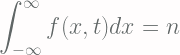
To implement a 1-D simulation of random walk $S(t)$ within period $t \in T = \{0, 1, 2, \dots, N\}$ in sample space $\omega \in \mathbb{W}$ , with discrete stochastic process $X_T = \{X_1, X_2, \dots, X_n \}$ called steps of the random walk with the constrain $\text{min} \leq X(t) \leq \text{max}$ .

Formulation

The random walk can be formally defined as follow:

$\displaystyle S(t) = S_0 + \sum_{t=1}^{n} X_t$

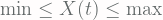$S_0$ represents the initial value or start point of the random walk. Also, select that each elements of $X_T$ can take on integer values between -5 and 5.

Implementation

This simulation is equivalent to plotting $S(t)$ against $t$ .

import numpy as np
import matplotlib.pyplot as plt

# Generate random numbers within the range -5 to 5
# Note that randint(-5, high=6) generate range -5 to 5
N =5100 ; MIN_STEP = -5; MAX_STEP = 6; S_0 = 0; # Define parameters of the simulation
X_T = np.random.randint(MIN_STEP , high=MAX_STEP , size=N+1) # Generate the discrete stochastic process
t = np.linspace(0, N, N+1) # Time domain
S = [S_0 + np.sum(X_T[0:i]) for i in xrange(N+1)] # Calculate each S(t) of the random walk
plt.plot(t, S, '-') # Plot

2D Random Flight

Further Discussions

In this example, we select that each elements $X(t) \in X_T, t \in T = \{0, 1, 2, \dots, n\}$ to follows $-5 \leq X(t) \leq 5 \text{ } \forall \text{ } t \in T$ . It is, however, possible to introduce various other constrain to the process w.r.t. the application of your application.

It is also worthwhile to note that both $S$ and $X_T=\{T_1, T_2, \dots, T_n\}$ fulfills the definition of stochastic process with the state space being different.

Learning Notes

Stochastic – Incremental Process

Posted on March 10, 2017March 14, 2017 by teracamo

Independent Incremental Process

For a stochastic process $X_T$ with sample space $t_1, t_2, \dots, t_n \in T$ such that $t_1 < t_2 < \dots < t_n$ then

$\displaystyle X_{t2} - X_{t1} , X_{t3} - X_{t2} , \dots , X_{tn} - X_{tn-1}$

are independent.

Stationary Independent Incremental Process

For an independent incremental process $X_T$ , it is said to be stationary if it satisfy:

$\displaystyle \{X_{t_i + h} - X_{t_{i-1} + h}\} = \{X_{t_i} - X_{t_{i-1}}\}$

A stationary independent incremental process is also called Levy Process

	Stochastic – P… on Stochastic – Poisson Pro…
	Anonymous on Stochastic – Poisson Pro…
	Stochastic – P… on Stochastic – Stationary…
	Stochastic – P… on Stochastic – Python Exam…
	Stochastic – P… on Stochastic Process

Introduction

Chapman-Kolomogov Equation

Differential Chapman-Kolomogov Equation

Assumptions

Derivation

Interpreting the equation

Discontinuous jumps

Fokker-Planck Equation

Reference

Definition of Problem

Annotation

Derivation

See Also

Taylor Series

Bra-kets Notation

Probabilities

Bayes’ theorem

Mean/Expectation value

Corelations

Covariance

Moments

Domain Transforms

Fourier Transform

Laplace Transform (Z-Transform)

Definition of Problem

Annotation

Derivation

Reference

See Also

Markov Property

Transition Probability Matrix

Transition Property of Markov Chain

Transition Probability written as Matrix

Example:

Properties of TPM

Prerequisite

Syntax

Poisson Distribution

Poisson Process

Definition

Example – Simulation of Poisson processes

Further Elaboration of results

Evolution of Poisson process

See Also

Definition of Problem

Annotation

Derivation

Side Notes

Reference

See also

Simple Random Walk

Defining the problem

Formulation

Implementation

2D Random Flight

Further Discussions

Independent Incremental Process

Stationary Independent Incremental Process

See Also