Annotation

$p(x, t|x_0, t_0)$ = Transition probability from state (x_0, t_0) to (x, t)

$g(s, t)$ = Generating function

$W(t)$ = Sample path of a Wiener process

Definition

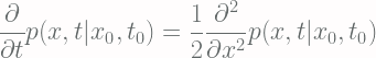
The definition of Wiener process is derived from the Fokker-Planck Equation, where the jump term of the master equation (or the Differential Chapman-Komogorov Equation) vanishes, and the coefficient of drift term A is zero and of diffusion term B is 1 [Eq.1]:

$\displaystyle \frac{\partial}{\partial t} p(x,t |x_0, t_0) = \frac{1}{2}\frac{\partial^2}{\partial x^2} p(x, t|x_0, t_0)$

A Wiener process is a Markov process which transitional probabilities fufill the upper equation.

Solving the PDE

Introduce the generating function [Eq.2]:

$\displaystyle g(s, t) = \int dx \big[ p(x, t|x_0, t_0) e^{isx} \big]$

and also the Bra-ket notation, defined as follow:

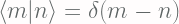
$\displaystyle \langle m | n \rangle = \delta (m-n)$
(Orthogonality)

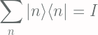
$\displaystyle \sum_n |n\rangle \langle n| = I$
(Completeness)

A Bra or ket are often referred as “basis”, because of the properties stated above, it is clear that once you define one of the basis, you can readily construct the other complement basis.

Rewriting the generating function:

$\displaystyle | x \rangle = e^{isx}$

$\displaystyle | g(s, t) \rangle = \int dx \big[ |x \rangle p(x, t|x_0, t_0) \big]$

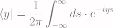
The complement basis can be defined as follow w.r.t the definition of Dirac-Delta function:

$\displaystyle \langle y | = \frac{1}{2\pi} \int_{-\infty}^{\infty} ds \cdot e^{-iys}$

The generating function is selected so that when combined with [Eq.1] (i.e. the Fokker-Plank Equation) such that satisfies the following:

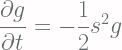
$\displaystyle \frac{\partial g}{\partial t} = -\frac{1}{2} s^2 g$

$\displaystyle | g \rangle = \exp ( -\frac{1}{2} s^2 t ) |g \rangle$
(solve by separation of variables)

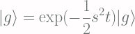
Consider the initial condition: 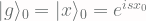$|g \rangle_0 = |x \rangle_0 = e^{isx_0}$ , we can solve for g(s, t):

$\displaystyle | g(s, t) \rangle = \exp \big[-\frac{1}{2}s^2(t - t_0)\big] | x \rangle_0$

Then by the property of Bra-ket:

$\displaystyle \langle y | g(s, t) \rangle = p(y, t|x_0, t_0)$

$\displaystyle p(y, t|x_0, t_0) = \frac{1}{2\pi} \int_{-\infty}^{\infty} ds \Big[ e^{-isy} e^{isx_0} \exp \big[ -\frac{1}{2}s^2(t - t_0) \big] \Big]$

$\displaystyle \indent = \frac{1}{2\pi} \int_{-\infty}^{\infty} ds \Big[ \exp \big[ -isy + isx_0 -\frac{1}{2}s^2(t - t_0) \big] \Big]$

Using integration by parts, we finally obtain the transition probability [Eq.3]:

$\displaystyle p(x, t|x_0, t_0) = \frac{1}{\sqrt{2\pi(t-t_0)}} \exp \left[ -\frac{(x-x_0)^2}{2(t-t_0)} \right]$

Interpretation of result

One can easily identify that the transitional probability is a Gaussian, then the actual process follows [Eq.3] and will have center and variance as follow:

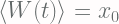
$\displaystyle \langle W(t) \rangle = x_0$

$\displaystyle \langle [W(t) - x_0]^2 \rangle = t - t_0$

Reference

Gardiner, C. “Stochastic methods: a handbook for the natural and social sciences 4th ed.(2009).”

	Stochastic – P… on Stochastic – Poisson Pro…
	Anonymous on Stochastic – Poisson Pro…
	Stochastic – P… on Stochastic – Stationary…
	Stochastic – P… on Stochastic – Python Exam…
	Stochastic – P… on Stochastic Process

Learning Records